How Phasers Work

Have you ever wondered what lies behind the intriguing wobbles and lush swooshes of this classic effect?

The popularity of the classic phaser effect might wax and wane, but it is an instantly familiar sound to every musician and, as our own Eddie Bazil demonstrated so well in a recent SOS Podcast (https://sosm.ag/UsingPhaserEffectsPodcast), it’s a far more powerful production tool than most of us realise. This article explains the technology that underpins the phaser, and explores several aspects of its mysterious but ingenious design.

Flanging First

Diagram 1. Both flangers and phasers work by splitting the signal in two, then processing one before recombining the signals.We’ll start with the simpler workings of the closely related flanger effect. Although there are tonal similarities between phasing and flanging, and they both employ similar architectures, their underlying technologies are actually rather different. Both effects use a signal path which splits the input signal to feed a processing path, the output of which is then recombined with the original signal to create the effected output, as shown in Diagram 1.

In a flanger, the processing element is a short delay, which is typically under 20 milliseconds. This obviously time‑shifts the signal slightly, which means that when it is recombined with the original, the alignment results in exactly opposite polarity for signals at a frequency related to the delay time (see Diagram 2). Crucially, though, there are further cancellations at all the octave multiples of that first frequency. In between those cancellations, the direct and delayed signals align in exactly the same polarity, so add together to boost the signal level. This arrangement produces a linear phase‑shift — in other words, a phase shift which doesn’t change with frequency.

Diagram 2. When mixing a delayed (and otherwise unprocessed) version of a signal with the original, there will be complete cancellation of some frequencies.

The result of combining a delayed signal with itself is an extended series of harmonically related notches and peaks in the overall frequency response, and we call this a ‘comb‑filter’ because the frequency response looks rather like a hair comb (Diagram 3). A 1ms delay will create a first notch at 500Hz, while a longer delay time lowers the frequency of the first notch, and vice versa (5ms gives a first notch at 100Hz, while 0.1ms would start at 5kHz, as per Diagram 3). Altering the mix proportions of original and delayed signals adjusts the depth of the notches and peaks, and many flangers also use feedback around the delay to increase the density and strength of the effect. Varying the delay time cyclically over a small range makes the notches/peaks move up and down the frequency spectrum to create that familiar ‘whooshing’ or ‘swirling’ effect.

Diagram 3. Comb‑filtering due to a 5 millisecond delay on one of two identical signals.

Phasing

A Phaser works in a very similar way to a flanger, but the first big difference is that it has only a few (usually, though not always, between two and six) notches rather than dozens of them, and the second is that these notches aren’t harmonically related to each other. The notches are still made to move up and down the spectrum in a similar way, though, and the result is typically a much more obvious and distinctive effect.

Instead of using a straight delay the Phaser’s core technology is the rather mysteriously named ‘all‑pass filter’, which is designed to introduce a polarity inversion at one frequency, to create a single notch in the frequency response; it doesn’t produce the harmonic series of notches that we saw in the flanger. In practice, two or three such notch filters are needed to optimise the effect, and that is achieved by using additional all‑pass filter stages daisy‑chained together... but we’re getting ahead of ourselves!

The frequency selectivity needed to create a single notch filter is achieved by shifting only the phase of the signal (hence the name) rather than its overall timing: a subtle but very important difference. By arranging the phase shift to reach 180 degrees at a specific frequency, combining this signal with the original results in a cancellation at only that frequency. To better understand how this phase‑shifting process works, we need to look at some basic electronic theory.

All Things Will Pass!

We are very used to thinking of filters and equalisers as things that change the amplitude of the signal over a specific range of frequencies, as displayed in ‘frequency response’ graphs. However, there is another side to (analogue) filters, which is that they also change the phase of the signal — meaning that some frequencies are fractionally delayed with respect to others in a non‑linear way. In other words, the phase plot has a curved response line, rather than straight.

Diagram 4. Analogue high‑ and low‑pass filters have an impact on the phase of signals that pass through them.

In a simple, first‑order, low‑pass filter, the high frequencies lag behind the low frequencies, while in a first‑order high‑pass filter the low frequencies lead the highs (see Diagram 4). We don’t usually bother to plot filter and EQ phase responses, because our sense of hearing doesn’t usually notice their effects — it’s the amplitude changes which grab most of our attention. Nevertheless, phase shifts are a fact of (analogue) filter design, and a fundamental pillar in the workings of a phaser.

Diagram 5. An all‑pass filter can be thought of as both a high‑ and low‑pass filter with the same turnover frequency operating in parallel, so that all frequencies pass through but the composite signal’s phase is altered.Low‑ and high‑pass filters are hopefully familiar terms, but earlier I mentioned something mysterious called an ‘all‑pass filter’. This is a special‑case filter that lets all frequencies through without changing their amplitude at all. So it’s not really a ‘filter’ in the conventional sense! But an all‑pass filter does change the phase of the signal at different frequencies, which is exactly what’s needed in a phaser.

Conceptually, an all‑pass filter is a bit like having both a high‑pass filter and a low‑pass filter working in parallel, with their outputs summed together. If their turnover frequencies were aligned, low frequencies would travel through the low‑pass route, and high‑frequencies through the high‑pass route, with the overall frequency response remaining completely flat. However, the phase of the output signal would vary considerably (and non‑linearly) with frequency.

A simpler form of this idea is a filter network comprising a capacitor and a resistor in parallel, but only joined together at their output ends. Conceptually, if you were to ground the resistor input the network resembles a first‑order high‑pass filter, and if you were to ground the capacitor input, a first order low‑pass filter. However, rather than grounding inputs, we are going to feed both with the same signal, but in opposite polarities (Diagram 5).

The impedance of a capacitor is very high for low frequencies, but reduces as the frequency rises. At low frequencies, the impedance of the capacitor is much higher than that of the resistor, so most of the inverted signal is passed through the resistor. Conversely, at high frequencies, the impedance of the capacitor is much lower than that of the resistor, so most of the (non‑inverted) signal now travels through the capacitor. (See the 'Voltage Vector' box for a fuller description of what’s going on here.)

In this way, all frequencies find a way through this resistor/capacitor network, and their varying strengths, combined with the phase shifts of the capacitor route, interact to ensure that the output sum of the two paths maintains the same overall amplitude as the original input signal. Critically, though, the phase shift through the network varies continuously with frequency, from 0 to 180 degrees, and at the frequency where the capacitor’s impedance exactly matches the value of the resistor, the phase shift is precisely 90 degrees.

Shin-Ei Uni-Vibe phaser. Diagram 6. The Shin‑Ei Uni‑Vibe’s two transistor‑based all‑pass filters are modulated by LFOs. I’ve simplified the all‑pass stages here, to show how the two transistors drive the resistor and capacitor stages with opposite signal polarities.

You’ll recall that we need a 180‑degree phase shift at the desired frequency to create a complete cancellation with the input signal, to form the notch filter. That’s easily achieved by chaining two of these simple all‑pass filter stages together, although in practice each stage needs to be electronically buffered to prevent unwanted interactions between them. The configuration described above is exactly how the classic Shin‑Ei Uni‑Vibe phaser works (see Diagram 6). It uses a specific configuration of paired transistors (called a Darlington Pair) to serve both as the stage buffer and to drive the resistor and capacitor network with opposite signal polarities. The output of the filter network feeds the next stage’s Darlington pair buffer. As we’ve seen, two all‑pass filter stages provide the 180‑degree phase shift needed to create one notch filter.

An alternative all‑pass filter configuration flips this circuit around, so it’s back to front. In the Uni‑Vibe design, the inverted signal through the resistor (‑R) is added to the signal through the capacitor (+C) to give us the sum: ‑R+C. Mathematically, that’s exactly the same as C‑R, and that can be done very easily with an op‑amp, thanks to its differential (inverting and non‑inverting) inputs. So in this alternative arrangement, the input signal feeds the junction of the resistor and capacitor, and their separate outputs feed the two inputs of an op‑amp, with the resistor feeding the subtractive (negative) input. The result is exactly the same, with each filter/op‑amp stage producing a 90‑degree phase shift at the frequency where C=R, so two stages are still needed to create a single notch filter (as shown in Diagram 7, below).

The MXR Phase 100 is unusual in that only three pairs of all‑pass stages receive the control signal to vary the filter notch frequency.

Sweeper System

So, we now know how to make a single notch filter using a pair of all‑pass filters, but we need to move that notch up and down in frequency. So how can we achieve that? Well, we know the notch frequency occurs when both all‑pass filters produce 90‑degree phase shifts, and that’s when the capacitor and resistor paths have equal impedance. So if we were to change the values of the resistors, we would change the notch frequency, and there are several readily available technologies to do just that.

Diagram 7. A simplified diagram of the classic MXR Phase 90’s dual op‑amp‑based all‑pass filter stages. For instance, we could replace the resistors in the all‑pass filters with a form of light‑dependent resistor (LDR) called a Vactrol. By shining a varying amount of light on the LDRs their resistances are altered. This is the approach taken in the Uni‑Vibe (again, see Diagram 6) and the Mu‑Tron Bi‑Phase. Alternatively, we could use a Junction‑FET (J‑FET) as the variable resistor, since the resistance between its Source and Drain terminals can be controlled by the voltage applied to the Gate terminal, and this is how the MXR Phase 90 and Phase 100 do it, although, for technical reasons, the J‑FET is used in practice as a potential divider in the capacitor arm. (Again, see Diagram 7.)

A more sophisticated solution involves the use of ‘operational transconductance amplifiers’ (OTAs). Whereas a standard op‑amp produces an output voltage proportional to the voltage difference between its two inputs, an OTA instead provides an output current proportional to the voltage difference and, importantly, that output current can be scaled by applying an external bias current. In other words the OTA acts like a variable resistance controlled by an external bias signal. The Electro Harmonix Small Stone Phaser (see Diagram 8) uses this technology, as does the Moog MoogerFooger MF‑103.

Diagram 8. The EHX Small Stone’s dual all‑pass filter stage, an example of a circuit which employs operational transconductance amplifiers, whose output can be scaled by a bias current. 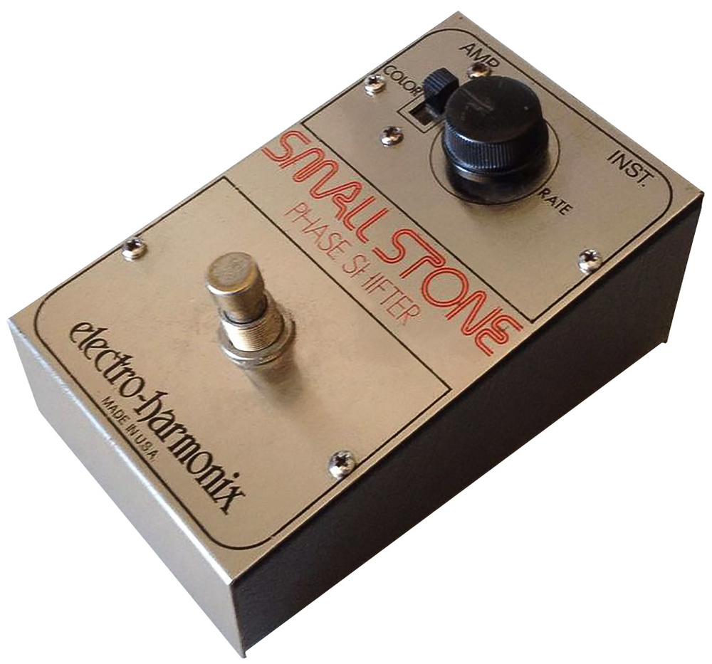Obviously, whatever technology is used to vary the notch frequencies, some form of control signal is required. Almost always, the main control source is a low‑frequency oscillator, usually with options to adjust its rate and depth, and sometimes its waveform shape as well. But as anyone who has dabbled in synthesis will know, plenty of other sources can be used as control signals, including audio signals.

Several pedals, such as the Boss PH‑3, offer an external input to allow that and/or to cater for expression pedal control. And as early as 1974, the Roland AP‑5 Phase Five (a precursor to the AP‑7 Jet Phaser, with its built‑in fuzz circuit) offered a touch‑sensitivity mode, in which the input signal’s amplitude determined the intensity of the phasing. LFOs and other synth‑style control options should be familiar as a concept to SOS readers, though, so I won’t dive deeper into that side of things here.

The Roland AP‑5 was one of the first phasers to use the input signal (and thus the playing dynamic) as the control source.

Adding More Notches & Feedback

When it comes to choosing a phaser, the aspect of the design which has arguably the greatest bearing on its sound character is how many notches are used, but how wide and deep those notches are is also important. Most classic guitarists’ phasers, including the MXR Phase 90, the Uni‑Vibe, and the EHX Small Stone, use a four‑stage all‑pass filter, which produces two moving notch filters. These pedals give a very obvious and pronounced sweeping coloration of the input signal.

The Moog Moogerfooger MF103 offers more filter stages than most, for a ‘thicker’ effect, but you can select fewer if that sounds too much.As explained earlier, though, flangers, with their very large number of notch filters, give a smoother‑sounding effect, so it’s perhaps not surprising that some phasers employ more notches to give a richer effect. For example, the MXR Phase 100 has 10 stages, creating five notches, and there are also models which allow you to select the number of stages. For instance, the Moog MF103 can be switched between six or 12 stages, giving either three or six notches, and the Maxon PH‑350 Rotary Phaser offers four, six or 10 stages, for two, three or five notches. (Of course, there are plenty of software phaser plug‑ins too, and some allow you to specify many more stages.)

In most cases, all of the filter stages receive the same LFO control signal, so all the notches track up and down together. However, the MXR Phase 100 is unusual in that only three pairs of all‑pass stages receive the control signal to vary the filter notch frequency. The other two notch filters remain static, and while their lack of movement means they’re not audible as such, their interaction with the three moving bands results in a very lush effect.

Adding feedback into the equation, with some of the processed signal being fed back to the input, changes the shape of the phaser’s notch filters, and many hardware and most software phasers will allow you to control this. As Diagram 9 shows, the more feedback you add, the less sharp and shallower the notches become, while the ‘mounds’ between the notches get narrower and peakier; the practical result is that wider frequency regions are attenuated, but not by as much.

Diagram 9: This plot shows the EHX Bad Stone Nano, a six‑stage phaser (so it produces three ‘notches’), using a range of different feedback settings from off to maximum. The higher the feedback control is set, the peakier the peaks and the deeper the dips! So increasing feedback essentially exaggerates the phasing effect.

So, there you have it: the inner workings of both phasing and flanging, and the enigmatically named all‑pass filter have hopefully now been demystified. If I’ve awakened your interest in phasing, I recommend listening to Eddie Bazil’s SOS Podcast that I mentioned at the outset; he takes you through some very impressive and unusual techniques.